Comparing Annual Returns of Bitcoin (BTC) and S&P 500 (SPY) Over the Last Decade

In the world of finance, understanding asset performance is key. Investors constantly weigh the potential rewards of high-growth, volatile assets like cryptocurrencies against the stability and historical performance of traditional markets represented by indices like the S&P 500.

In this post, we’ll dive into a practical analysis using Python to compare the annual returns of Bitcoin (BTC) and the SPDR S&P 500 ETF Trust (SPY) over the past 10 years. This analysis will shed light on their respective performance characteristics during a significant period of market evolution, including the rise of digital assets.

We’ll walk through:

• Why compare BTC and SPY?
• How to fetch historical financial data using Python.
• Calculating annual returns.
• Visualizing the results.
• Interpreting the findings for your investment perspective.

This is a great way to apply your Python skills to real-world financial data analysis. Let’s get started!

Why Compare Bitcoin and the S&P 500?

Bitcoin, as the pioneer and largest cryptocurrency, represents the burgeoning digital asset class, known for its high volatility and potential for exponential growth. The S&P 500, on the other hand, is a benchmark index representing 500 of the largest U.S. publicly traded companies, widely considered a proxy for the overall U.S. stock market’s health and a cornerstone of traditional investment portfolios.

Comparing their annual returns over a substantial period like 10 years allows us to contrast the performance of a nascent, disruptive technology asset against established equity markets. It helps illustrate the risk-reward profiles and diversification potential (or lack thereof) when considering both in a portfolio.

Getting the Data with Python

To perform this analysis, we need historical price data for both BTC and SPY. The yfinance library in Python is an excellent tool for this, allowing us to download data directly from Yahoo Finance. We’ll also use pandas for data manipulation and matplotlib or plotly for visualization.

First, ensure you have the necessary libraries installed:

pip install yfinance pandas matplotlib plotly

We will fetch the adjusted close prices for both assets. Adjusted close price is important as it accounts for dividends and stock splits, providing a more accurate picture of the asset’s value over time.

Calculating Annual Returns

Once we have the daily price data, we can calculate the daily returns. The daily return is simply the percentage change in price from one day to the next.

Daily Return = (Current Day Price−Previous Day Price)/Previous Day Price

To get the annual return, we can’t just average the daily returns. Instead, we typically calculate the cumulative return over the year and then express it as a percentage. A simpler approach for annual returns is to calculate the percentage change from the last trading day of the previous year to the last trading day of the current year.

We will resample the data to an annual frequency and calculate the percentage change year-over-year.

import yfinance as yf
import pandas as pd
import matplotlib.pyplot as plt

# Define the tickers and date range
tickers = ["BTC-USD", "SPY"]
start_date = "2014-04-23"
end_date = "2025-04-23"

print(f"Fetching data for {tickers} from {start_date} to {end_date}...")

try:
    # Download historical data using yfinance
    data = yf.download(tickers, start=start_date, end=end_date)['Close']

    if data.empty:
        print("Error: Could not download data. Please check tickers and date range.")
    else:
        print("Data downloaded successfully.")

        # Calculate annual returns using a better approach
        # First, resample to get the last trading day of each year
        # Use 'A' for annual frequency which gives the last day of each year
        yearly_prices = data.resample('A').last()
        
        # For more accurate returns, also get the first trading day of each year
        # to calculate year-over-year returns
        annual_returns = yearly_prices.pct_change() * 100

        # Drop the first row which will contain NaNs due to pct_change
        annual_returns = annual_returns.dropna()

        # Rename columns for clarity
        annual_returns.columns = ['Bitcoin (BTC)', 'S&P 500 (SPY)']

        print("\nCalculated Annual Returns (%):")
        print(annual_returns)

        # Plotting the annual returns
        plt.figure(figsize=(12, 7))
        bar_width = 0.35
        index = annual_returns.index.year

        # Plot bars for Bitcoin
        plt.bar(index - bar_width/2, annual_returns['Bitcoin (BTC)'], 
                bar_width, label='Bitcoin (BTC)', color='orange')
        # Plot bars for SPY
        plt.bar(index + bar_width/2, annual_returns['S&P 500 (SPY)'], 
                bar_width, label='S&P 500 (SPY)', color='blue')

        plt.xlabel('Year')
        plt.ylabel('Annual Return (%)')
        plt.title('Annual Returns of Bitcoin (BTC) vs S&P 500 (SPY) (Last 10 Years)')
        plt.xticks(index)
        plt.axhline(0, color='grey', linestyle='--', linewidth=0.8)
        plt.legend()
        plt.grid(axis='y', linestyle='--', alpha=0.7)
        plt.tight_layout()
        plt.show()

except Exception as e:
    print(f"An error occurred: {e}")

Visualizing the Results

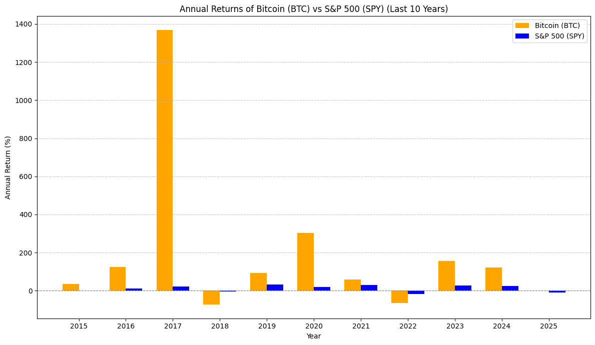
A picture is worth a thousand words, especially in data analysis. We will create a bar chart comparing the annual returns of BTC and SPY side-by-side for each year. This visualization will make it easy to see the year-to-year performance differences and the periods where one asset significantly outperformed the other.

Interpreting the Findings

After running the code and visualizing the returns, we can analyze the results. We’ll look for patterns such as:

• Which asset had higher average annual returns?
• Which asset exhibited greater volatility (larger swings in annual performance)?
• Were there specific years where the performance diverged significantly?
• How did the performance compare during bullish or bearish market periods?

This analysis is for educational purposes and should not be considered financial advice. Past performance is not indicative of future results.

Here are some key observations:

1. Bitcoin’s Extreme Volatility and High Peaks: Bitcoin has experienced several years of exceptionally high returns, notably in 2017 where its annual return soared dramatically. However, it also shows significant negative returns in other years, such as 2018 and 2022. This visually emphasizes Bitcoin’s high volatility and boom-and-bust cycles.
2. S&P 500’s Consistent, Positive Returns: In contrast, the S&P 500 has shown much more consistent, albeit generally lower, positive annual returns over the decade. There are very few years with negative returns for SPY in this period, and the magnitude of these negative returns is much smaller than Bitcoin’s downturns.
3. Divergence in Performance: The chart highlights years where the performance of the two assets diverged significantly. For instance, in 2017, Bitcoin’s massive gains dwarfed SPY’s positive return. Conversely, in a year like 2018, when Bitcoin saw a large loss, SPY still posted a positive return.
4. Risk-Reward Trade-off: The visual comparison underscores the classic risk-reward trade-off. Bitcoin offered the potential for much higher returns but came with considerably greater risk due to its volatility. The S&P 500 provided more stability and consistent growth, suitable for investors with lower risk tolerance.

The Python Code Explained (High-Level)

The Python script performs the following key steps:

1. Import Libraries: Imports yfinance, pandas, and matplotlib (or plotly).
2. Define Tickers and Date Range: Specifies the Yahoo Finance tickers for BTC (BTC-USD) and SPY (SPY), and sets the start and end dates for the 10-year period.
3. Download Data: Uses yfinance.download() to fetch the historical adjusted close price data for both tickers within the specified date range.
4. Calculate Annual Returns:
   • Resamples the daily data to annual frequency, taking the last trading day’s price for each year.
   • Calculates the year-over-year percentage change using the .pct_change() method.
   • Multiplies by 100 to express returns as percentages.
5. Combine Data: Merges the annual returns for BTC and SPY into a single pandas DataFrame for easier plotting.
6. Plot Results: Creates a bar chart using matplotlib (or plotly) to visualize the annual returns side-by-side. Adds titles, labels, and a legend for clarity. Displays the plot.

This script provides a clear and concise way to perform the annual return comparison programmatically.

Conclusion

Analyzing the annual returns of Bitcoin and the S&P 500 over the last decade reveals fascinating insights into the performance characteristics of these two vastly different asset classes. While Bitcoin has demonstrated periods of explosive growth, it has also experienced significant downturns, highlighting its higher risk profile compared to the more stable, albeit generally lower-returning, S&P 500.

Understanding these historical trends is crucial for investors building diversified portfolios and making informed decisions based on their risk tolerance and investment goals. Python provides powerful tools to conduct such analyses efficiently.

Stay tuned for more Python for Finance tutorials!

Disclaimer: This article is for informational and educational purposes only and does not constitute financial advice. . Always conduct thorough due diligence or consult a qualified financial advisor before making investment decisions. This blog post was drafted with the assistance of AI tools and reviewed and edited by the author.