1. Building a Simple Portfolio with Python and Real-World Data

Portfolio management is a crucial skill for any investor, whether you’re managing your own savings or working in finance. At its core, portfolio management is about balancing risk and return to achieve your financial goals. With the rise of powerful tools like Python, even beginners can dive into this world and start analyzing real-world data with just a few lines of code.

In this post, we’ll walk through the basics of portfolio management using Python. We’ll fetch real stock data from Yahoo Finance, build a simple portfolio, and visualize how a $10,000 investment would have performed over a year. By the end, you’ll have a solid foundation to explore more advanced techniques.

Introduction: Why Python for Portfolio Management?

Python is a fantastic tool for portfolio management because of its simplicity and the vast ecosystem of libraries tailored for data analysis and finance. Whether you’re a beginner or an experienced programmer, Python makes it easy to fetch, analyze, and visualize financial data.

In this post, we’ll use yfinance, a popular library that allows us to download historical stock prices directly from Yahoo Finance. We’ll focus on three well-known stocks—Apple (AAPL), Microsoft (MSFT), and Amazon (AMZN)—and build a portfolio that assumes equal investment in each. By the end, you’ll see how this portfolio would have grown over a year compared to investing in each stock individually.

Key Concepts: Portfolio Return and Risk

Before we dive into the code, let’s cover two fundamental concepts:

• Portfolio Return: This is the profit or loss generated by your portfolio, usually expressed as a percentage. It’s calculated based on the weighted returns of the individual assets (like stocks) in your portfolio.
• Portfolio Risk: Risk refers to the uncertainty or variability of returns. In finance, it’s often measured by standard deviation (also known as volatility). A higher standard deviation means more risk, as the portfolio’s value can fluctuate more dramatically.

One of the key strategies in portfolio management is diversification—spreading your investments across different assets to reduce risk. By combining assets that don’t move in perfect unison (i.e., they have low or negative correlation), you can potentially lower the overall risk without sacrificing too much return.

In this post, we’ll build a simple portfolio with three stocks to see diversification in action.

Step-by-Step Implementation: Building the Portfolio

Let’s walk through the process of building and analyzing a portfolio using Python. We’ll use real data from Yahoo Finance and break everything down into easy-to-understand steps.

Step 1: Fetching Data with yfinance

First, we need historical stock prices. We’ll use the yfinance library to download adjusted closing prices for AAPL, MSFT, and AMZN from January 1, 2022, to January 1, 2023.

import yfinance as yf
import pandas as pd
import numpy as np
import matplotlib.pyplot as plt

# Define the stocks and the period
tickers = ['AAPL', 'MSFT', 'AMZN']
start_date = '2022-01-01'
end_date = '2023-01-01'

# Download adjusted closing prices
data = yf.download(tickers, start=start_date, end=end_date)['Close']

• What’s happening here?
  We’re downloading the adjusted closing prices, which account for dividends and stock splits, giving us a more accurate picture of each stock’s performance.

Step 2: Calculating Daily Returns

Next, we calculate the daily percentage returns for each stock. This tells us how much each stock’s price changed from one day to the next.

# Calculate daily returns
returns = data.pct_change().dropna()

• What’s happening here?
  The pct_change() function computes the percentage change between consecutive days, and dropna() removes any missing values (like the first day, which has no prior data).

Step 3: Constructing the Portfolio

Now, we’ll assume an equal-weight portfolio, meaning we invest the same amount in each stock. For three stocks, each gets a weight of 1/3.

# Assume equal weights for each stock
weights = np.array([1/len(tickers)] * len(tickers))

# Calculate portfolio daily returns
portfolio_returns = returns.dot(weights)

• What’s happening here?
  We use the dot product of the stock returns and the weights to get the portfolio’s daily return. This is a weighted average of the individual stock returns.

Step 4: Calculating Portfolio Value Over Time

Let’s assume we start with a $10,000 investment. We’ll calculate how the portfolio’s value changes over time based on the daily returns.

# Calculate portfolio value over time, starting with $10,000
initial_investment = 10000
portfolio_value = initial_investment * (1 + portfolio_returns).cumprod()

• What’s happening here?
  We use the cumulative product of (1 + daily returns) to simulate how the investment grows (or shrinks) day by day.

Step 5: Visualizing the Results

Finally, we’ll plot the portfolio’s value over time and compare it to the performance of each individual stock.

# Plot the portfolio value and individual stock values
plt.figure(figsize=(10, 6))
portfolio_value.plot(label='Portfolio')
for ticker in tickers:
    stock_value = initial_investment * (1 + returns[ticker]).cumprod()
    stock_value.plot(label=ticker)
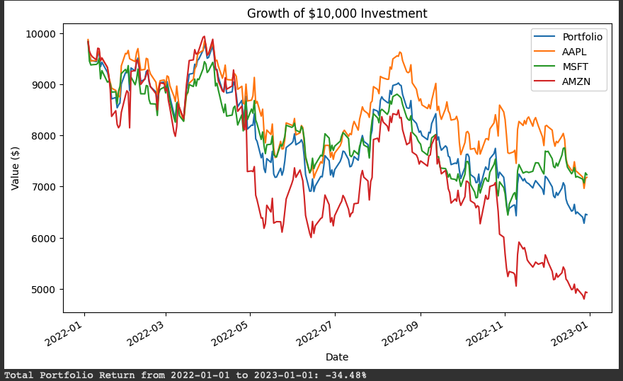
plt.title('Growth of $10,000 Investment')
plt.xlabel('Date')
plt.ylabel('Value ($)')
plt.legend()
plt.show()

• What’s happening here?
  This plot shows how a $10,000 investment in the portfolio would have performed compared to investing the same amount in each stock individually. It’s a great way to visualize the benefits of diversification.

Understanding the Results

When you run the code, you’ll see a plot with four lines: one for the portfolio and one for each stock. Here’s what you might observe:

• Portfolio Performance: The portfolio’s value likely fluctuates less than the individual stocks, especially if the stocks didn’t move in perfect sync during the year. This is diversification at work—it smooths out the ups and downs.
• Individual Stocks: Some stocks may have outperformed the portfolio, but others may have underperformed. The portfolio balances these outcomes, aiming for a more stable return.

To wrap up, let’s calculate the total return of the portfolio over the year.

# Calculate total portfolio return over the period
total_return = (portfolio_value.iloc[-1] / portfolio_value.iloc[0]) - 1
print(f"Total Portfolio Return from {start_date} to {end_date}: {total_return:.2%}")

This will give you the percentage return on your $10,000 investment. For example, if the portfolio grew to around $7,000, the total return would be -35%.

Conclusion: Actionable Takeaways

Congratulations! You’ve just built a simple portfolio using real-world data and Python. Here’s what you can do next to deepen your understanding:

• Experiment with Different Stocks: Try replacing AAPL, MSFT, and AMZN with other stocks or even ETFs. How does the portfolio’s performance change?
• Adjust the Weights: Instead of equal weights, try allocating more to one stock and less to others. Does this increase or decrease the portfolio’s risk and return?
• Explore Other Metrics: Look into calculating the portfolio’s volatility or the Sharpe ratio (a measure of risk-adjusted return) to get a fuller picture of performance.
• Automate Data Updates: Use Python to fetch the latest data daily or weekly, so you can track your portfolio’s performance in real-time.

Portfolio management is both an art and a science, and Python gives you the tools to explore it with confidence. Keep experimenting, and you’ll be well on your way to mastering the balance between risk and reward.