5. Python Portfolio Management: Building a Backtesting Framework

Welcome to the fifth article in our Python Portfolio Management series! So far, we’ve covered the basics of portfolio management, building efficient frontiers, implementing risk management techniques, and calculating beta and dollar sensitivity. Today, we’ll explore how to build a backtesting framework to evaluate the performance of your investment strategies using Python.

Backtesting is a critical step in portfolio management that allows you to simulate how your investment strategy would have performed using historical data. This helps you validate your approach before risking real capital.

Disclaimer: This article was drafted with the assistance of artificial intelligence and reviewed by the editor prior to publication to ensure accuracy and clarity.

Setting Up Our Environment

Let’s start by importing the necessary libraries:

import numpy as np
import pandas as pd
import matplotlib.pyplot as plt
import yfinance as yf
import seaborn as sns
from datetime import datetime, timedelta
from scipy import stats

# Set plotting style
plt.style.use('fivethirtyeight')
sns.set_palette("pastel")

Downloading Historical Data

First, we’ll create a function to download historical price data for our assets. For our example, we will take five of the most popular stocks. Below function will download the historical stock data for the selected tickers:

def get_stock_data(tickers, start_date, end_date):
    """
    Download historical stock data for the given tickers and date range

    Parameters:
    tickers (list): List of stock ticker symbols
    start_date (str): Start date in 'YYYY-MM-DD' format
    end_date (str): End date in 'YYYY-MM-DD' format

    Returns:
    DataFrame: Daily adjusted closing prices for each ticker
    """
    data = yf.download(tickers, start=start_date, end=end_date)['Adj Close']

    # If only one ticker is provided, convert Series to DataFrame
    if len(tickers) == 1:
        data = data.to_frame(name=tickers[0])

    return data

Creating a Basic Portfolio Backtesting Class

Now, let’s build a comprehensive backtesting class that will allow us to:

1. Define portfolio weights
2. Calculate daily returns
3. Track portfolio value over time
4. Generate performance metrics

class PortfolioBacktest:
    def __init__(self, price_data, weights=None, initial_capital=10000):
        """
        Initialize the backtesting framework

        Parameters:
        price_data (DataFrame): Historical price data with tickers as columns
        weights (dict): Dictionary mapping tickers to weights
        initial_capital (float): Starting capital for the backtest
        """
        self.price_data = price_data
        self.tickers = list(price_data.columns)

        # If no weights provided, use equal weights
        if weights is None:
            equal_weight = 1.0 / len(self.tickers)
            self.weights = {ticker: equal_weight for ticker in self.tickers}
        else:
            self.weights = weights

        self.initial_capital = initial_capital
        self.results = None

    def run_backtest(self, rebalance_freq='Q'):
        """
        Run the backtest with optional rebalancing

        Parameters:
        rebalance_freq (str): Rebalancing frequency:
                             'D' for daily, 'W' for weekly,
                             'M' for monthly, 'Q' for quarterly, 'Y' for yearly

        Returns:
        DataFrame: Daily portfolio values and metrics
        """
        # Calculate returns from prices
        returns = self.price_data.pct_change().dropna()

        # Initialize results dataframe
        self.results = pd.DataFrame(index=returns.index)

        # Create columns for each ticker's allocation and value
        for ticker in self.tickers:
            self.results[f'{ticker}_weight'] = 0
            self.results[f'{ticker}_value'] = 0

        self.results['portfolio_value'] = 0

        # Get rebalancing dates '''
Explanation: Below code uses the resample method on the returns object (which is expected to be a pandas DataFrame or Series with a DatetimeIndex).
The resample(rebalance_freq) call groups the return data into periods defined by rebalance_freq (for example, "M" for monthly, "W" for weekly, etc.).
The .first() method selects the first observed value in each of these periods, assuming that this represents the correct time to rebalance.
Finally, .index extracts the dates corresponding to these first values, resulting in a series of rebalancing dates.
'''
        if rebalance_freq:
            rebalance_dates = returns.resample(rebalance_freq).first().index
        else:
            # If no rebalancing, just use the first date
            rebalance_dates = [returns.index[0]]

        # Initialize portfolio
        current_value = self.initial_capital
        current_weights = self.weights
        shares = {}

        # Loop through each day in the backtest
        for date in returns.index:
            # Check if we need to rebalance
            if date in rebalance_dates or date == returns.index[0]: 
                # Calculate shares to hold based on current weights 
                #Once the code determines that a rebalance is needed, it calculates the number #of shares to hold for each asset (ticker) based on the current portfolio value and target #weights
                for ticker in self.tickers:
                    ticker_value = current_value * current_weights[ticker]
                    price = self.price_data.loc[date, ticker]
                    shares[ticker] = ticker_value / price

            # Update portfolio value for this day
            new_value = sum(shares[ticker] * self.price_data.loc[date, ticker] 
                           for ticker in self.tickers)

            # Record portfolio value
            self.results.loc[date, 'portfolio_value'] = new_value

            # Record individual ticker weights and values
            for ticker in self.tickers:
                ticker_value = shares[ticker] * self.price_data.loc[date, ticker]
                self.results.loc[date, f'{ticker}_value'] = ticker_value
                self.results.loc[date, f'{ticker}_weight'] = ticker_value / new_value

            # Update current value for next iteration
            current_value = new_value

        # Calculate daily returns
        self.results['daily_return'] = self.results['portfolio_value'].pct_change()

        # Calculate cumulative returns
        self.results['cumulative_return'] = (1 + self.results['daily_return']).cumprod() - 1

        return self.results

    def calculate_metrics(self):
        """
        Calculate performance metrics for the backtest

        Returns:
        dict: Dictionary of performance metrics
        """
        if self.results is None:
            raise ValueError("Backtest must be run before calculating metrics")

        daily_returns = self.results['daily_return'].dropna()

        # Annualization factors
        days_per_year = 252

        # Calculate metrics
        total_return = self.results['portfolio_value'].iloc[-1] / self.initial_capital - 1
        #daily_returns provide information about the number of days in the period
        annual_return = (1 + total_return) ** (days_per_year / len(daily_returns)) - 1
        annual_volatility = daily_returns.std() * np.sqrt(days_per_year)
        sharpe_ratio = annual_return / annual_volatility if annual_volatility != 0 else 0

        # Calculate max drawdown
        cumulative_returns = (1 + daily_returns).cumprod()
        peak = cumulative_returns.expanding().max()
        drawdown = (cumulative_returns / peak) - 1
        max_drawdown = drawdown.min()

        # Calculate Sortino ratio (downside deviation)
        negative_returns = daily_returns[daily_returns < 0]
        downside_deviation = negative_returns.std() * np.sqrt(days_per_year)
        sortino_ratio = annual_return / downside_deviation if downside_deviation != 0 else 0

        metrics = {
            'Total Return': total_return,
            'Annual Return': annual_return,
            'Annual Volatility': annual_volatility,
            'Sharpe Ratio': sharpe_ratio,
            'Max Drawdown': max_drawdown,
            'Sortino Ratio': sortino_ratio
        }

        return metrics

    def plot_performance(self, benchmark=None):
        """
        Plot portfolio performance

        Parameters:
        benchmark (DataFrame): Optional benchmark data with same index as results
        """
        if self.results is None:
            raise ValueError("Backtest must be run before plotting")

        fig, axes = plt.subplots(3, 1, figsize=(12, 15))

        # Plot 1: Portfolio Value Over Time
        self.results['portfolio_value'].plot(ax=axes[0])
        axes[0].set_title('Portfolio Value Over Time')
        axes[0].set_ylabel('Value ($)')
        axes[0].grid(True)

        # Plot 2: Asset Allocation Over Time
        weight_cols = [col for col in self.results.columns if col.endswith('_weight')]
        self.results[weight_cols].plot.area(ax=axes[1], stacked=True)
        axes[1].set_title('Asset Allocation Over Time')
        axes[1].set_ylabel('Weight')
        axes[1].set_ylim(0, 1)
        axes[1].legend([col.split('_')[0] for col in weight_cols])
        axes[1].grid(True)

        # Plot 3: Cumulative Returns (vs Benchmark if provided)
        self.results['cumulative_return'].plot(ax=axes[2], label='Portfolio')

        if benchmark is not None:
            benchmark_returns = benchmark.pct_change().dropna()
            cumulative_benchmark = (1 + benchmark_returns).cumprod() - 1
            cumulative_benchmark.plot(ax=axes[2], label='Benchmark')

        axes[2].set_title('Cumulative Returns')
        axes[2].set_ylabel('Return')
        axes[2].legend()
        axes[2].grid(True)

        plt.tight_layout()
        plt.show()

Using the Backtesting Framework

Now let’s put our framework to use with a practical example. We’ll create a portfolio of tech stocks and compare it against the S&P 500 index:

# Define tickers and date range
tickers = ['AAPL', 'MSFT', 'GOOGL', 'AMZN', 'META']
benchmark_ticker = 'SPY'  # S&P 500 ETF
start_date = '2018-01-01'
end_date = '2023-01-01'

# Download data
stock_data = get_stock_data(tickers + [benchmark_ticker], start_date, end_date)
portfolio_data = stock_data[tickers]
benchmark_data = stock_data[[benchmark_ticker]]

# Define custom weights (optional)
custom_weights = {
    'AAPL': 0.25,
    'MSFT': 0.25,
    'GOOGL': 0.20,
    'AMZN': 0.15,
    'META': 0.15
}

# Create and run backtest
backtest = PortfolioBacktest(portfolio_data, weights=custom_weights, initial_capital=10000)
results = backtest.run_backtest(rebalance_freq='Q')  # Quarterly rebalancing

# Calculate and display metrics
metrics = backtest.calculate_metrics()
for metric, value in metrics.items():
    print(f"{metric}: {value:.4f}")

# Plot performance against benchmark
backtest.plot_performance(benchmark=benchmark_data)

By running this Python code, we get to the results displayed in below picture. The portfolio starts with a value of around $10,000 in 2018 and grows steadily over time, peaking at over $30,000 in late 2021 or early 2022.

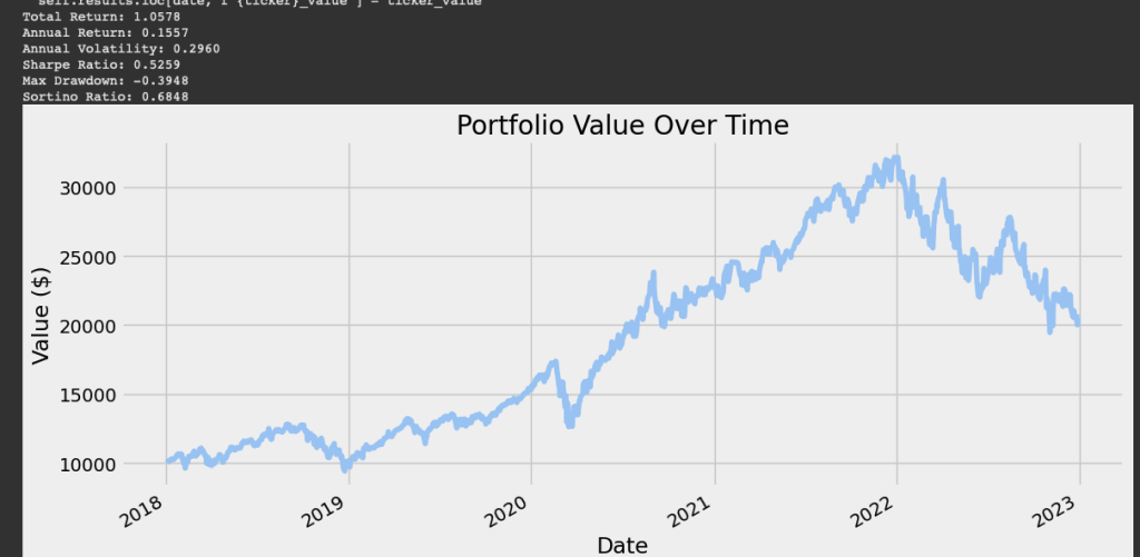
After the peak, the portfolio experiences a significant drawdown, losing value throughout 2022, before stabilizing in 2023. Some of the key metrics are as follows:

Total Return: 1.0578

• This indicates the portfolio grew by approximately 105.78% over the entire period. For example, if the initial investment was $10,000, it grew to $20,578 by the end of the period.

Annual Return: 0.1557 (15.57%)

• The portfolio achieved an average annualized return of 15.57%, which is strong and above the historical average of the S&P 500 (around 10% annually).

Annual Volatility: 0.2960 (29.60%)

• Volatility measures the portfolio’s risk or fluctuations in value. A 29.60% annual volatility is relatively high, indicating the portfolio experienced significant ups and downs. This level of volatility is typical for portfolios with exposure to equities or other high-risk assets.

Sharpe Ratio: 0.5259

• The Sharpe ratio measures risk-adjusted returns. A ratio of 0.5259 indicates that the portfolio generated returns, but not exceptionally well relative to the risk taken.
• A Sharpe ratio above 1 is considered excellent, while below 0.5 suggests the risk may not be adequately compensated by returns. This portfolio is in the middle range.

Max Drawdown: -0.3948 (-39.48%)

• The maximum drawdown of -39.48% indicates the portfolio lost nearly 40% of its value from its peak to its trough during the period.
• This is a significant drawdown and highlights the portfolio’s vulnerability to market downturns, particularly in 2022.

Sortino Ratio: 0.6848

• The Sortino ratio is similar to the Sharpe ratio but focuses only on downside risk. A ratio of 0.6848 suggests the portfolio performed moderately well in generating returns relative to the downside risk.
• A higher Sortino ratio (above 1) would indicate better downside risk management.

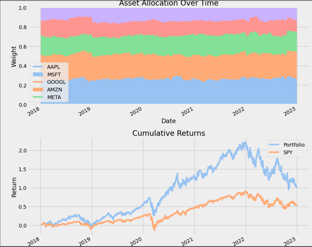
In addition, we also see displayed the asset allocation over time and the cumulative returns versus the SPY. The allocation appears to be relatively stable over time, with no significant rebalancing or changes in weights.

AAPL and MSFT consistently have the largest weights, making up a significant portion of the portfolio (approximately 40-50% combined).

GOOGL, AMZN, and META have smaller but still substantial allocations, each contributing around 10-20%.

Analyzing Drawdowns

Understanding drawdowns is crucial for risk management. Let’s add a function to analyze the worst drawdowns in our portfolio:

def analyze_drawdowns(backtest_results, top_n=5):
    """
    Analyze the top N worst drawdowns in the portfolio

    Parameters:
    backtest_results (DataFrame): Results from the backtest
    top_n (int): Number of worst drawdowns to analyze

    Returns:
    DataFrame: Drawdown statistics
    """
    # Calculate equity curve
    equity_curve = backtest_results['portfolio_value']

    # Calculate running maximum. The "equity curve" is the evolution of portfolio's value over #time
    running_max = equity_curve.cummax()
    '''
Explanation: The running maximum calculates the highest value the portfolio has reached up to each point in time. The cummax() method on the equity curve produces a new time series where each value is the maximum portfolio value observed up to that date
'''
    # Calculate drawdowns
'''
Explanation: The drawdown quantifies the percentage difference between the current portfolio value and the highest value it has achieved so far
'''
    drawdowns = (equity_curve / running_max - 1)

    # Find drawdown periods
    is_in_drawdown = drawdowns < 0

    # Label drawdown periods
    drawdown_number = (is_in_drawdown & ~is_in_drawdown.shift(1).fillna(False)).cumsum()

    # Group by drawdown periods
    grouped = pd.DataFrame({
        'drawdown': drawdowns,
        'equity': equity_curve,
        'period': drawdown_number
    }).groupby('period')

    # Calculate stats for each drawdown
    drawdown_info = []

    for period, group in grouped:
        if group['drawdown'].min() >= 0:
            continue

        recovery = group['equity'].iloc[-1] >= running_max.loc[group.index[0]]

        start_date = group.index[0]
        end_idx = group['drawdown'].idxmin() if not recovery else group.index[-1]
        recovery_date = group.index[-1] if recovery else None

        duration = (end_idx - start_date).days
        recovery_days = (recovery_date - end_idx).days if recovery else None

        drawdown_info.append({
            'Start Date': start_date,
            'Bottom Date': end_idx,
            'End Date': recovery_date,
            'Max Drawdown': group['drawdown'].min(),
            'Duration (Days)': duration,
            'Recovery (Days)': recovery_days,
            'Recovered': recovery
        })

    # Convert to DataFrame and sort by Max Drawdown
    drawdown_df = pd.DataFrame(drawdown_info)
    if len(drawdown_df) > 0:
        drawdown_df = drawdown_df.sort_values('Max Drawdown').head(top_n)

    return drawdown_df

# Usage
drawdowns = analyze_drawdowns(results)
print("\nWorst Drawdowns:")
print(drawdowns)

The output of this code is nice since it allows us to see when the worst drawdown happen for the selected portfolio. The worst Drawdown happened during 2022 with a down return of 39% from the peak:

Comparing Different Rebalancing Strategies

Let’s compare how different rebalancing frequencies affect portfolio performance:

def compare_rebalancing_strategies(price_data, weights, frequencies=['Y', 'Q', 'M', 'W']):
    """
    Compare portfolio performance with different rebalancing frequencies
    
    Parameters:
    price_data (DataFrame): Historical price data
    weights (dict): Portfolio weights
    frequencies (list): List of rebalancing frequencies to compare
    
    Returns:
    DataFrame: Performance metrics for each strategy
    """
    results = {}
    
    # Store each backtest result for validation
    backtest_results = {}
    
    for freq in frequencies:
        # Create description based on frequency
        if freq == 'Y':
            desc = 'Yearly'
        elif freq == 'Q':
            desc = 'Quarterly'
        elif freq == 'M':
            desc = 'Monthly'
        elif freq == 'W':
            desc = 'Weekly'
        else:
            desc = freq
            
        # Run backtest with this frequency
        backtest = PortfolioBacktest(price_data, weights=weights)
        backtest_results[desc] = backtest.run_backtest(rebalance_freq=freq)
        metrics = backtest.calculate_metrics()
        
        # Store results
        results[desc] = metrics
    

    
    # Verify that strategies are indeed different by checking final weights
    print("\nFinal portfolio weights:")
    for strategy, result in backtest_results.items():
        weight_cols = [col for col in result.columns if col.endswith('_weight')]
        final_weights = result[weight_cols].iloc[-1]
        print(f"{strategy}: {dict(zip([col.split('_')[0] for col in weight_cols], final_weights.values))}")
    
    # Convert to DataFrame for easy comparison
    results_df = pd.DataFrame(results)
    
    return results_df

# Usage
rebalancing_comparison = compare_rebalancing_strategies(portfolio_data, custom_weights)
print("\nRebalancing Strategy Comparison:")

print(rebalancing_comparison)

# Visualize the comparison
plt.figure(figsize=(12, 8))
rebalancing_comparison.loc[['Annual Return', 'Annual Volatility', 'Sharpe Ratio']].plot(kind='bar')
plt.title('Performance Metrics by Rebalancing Frequency')
plt.ylabel('Value')
plt.xticks(rotation=0)
plt.grid(axis='y')
plt.show()

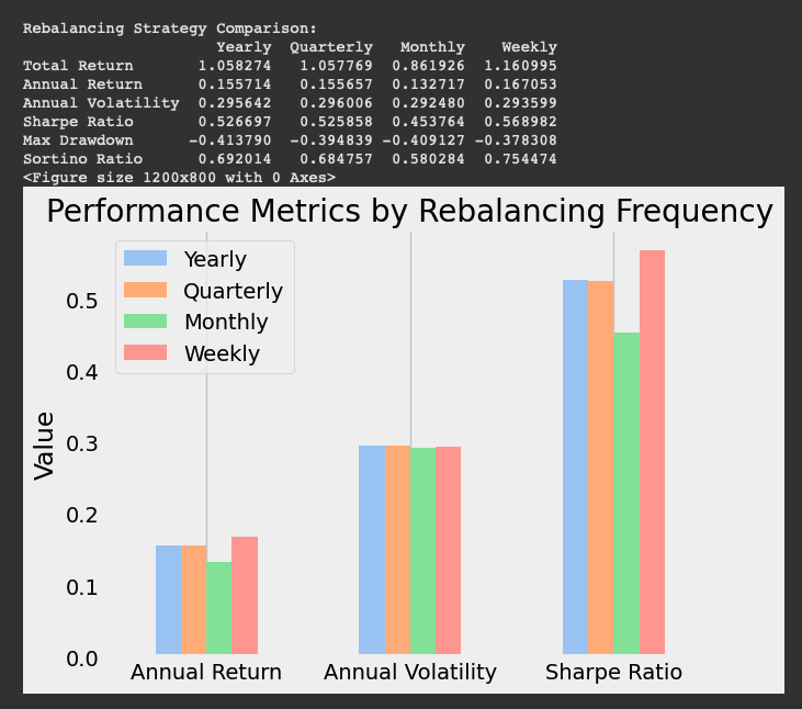
The rebalancing frequency also plays a role in our portfolio return as displayed with the code above. Weekly rebalancing seems to achieve the highest total return and the highest Sharpe ratio.

Testing Different Allocation Strategies

Finally, let’s compare different allocation strategies. Three portfolio allocation strategies are defined for our case:

Defensive approach:

Apple (AAPL), Google (GOOGL), and Amazon (AMZN) receive smaller weights, reflecting a more balanced and defensive approach within the tech sector. To be honest, the classification between high and defensive tech makes no sense, but let’s keep it like this for practical purposes only. You can define your own weights with your own stocks.

Equal Weight:

All assets are assigned equal weights. For example, if there are 5 assets, each gets a weight of 15=0.251​=0.2.

This strategy is simple and ensures no single asset dominates the portfolio.

High Tech:

This strategy focuses heavily on tech giants like Apple (AAPL) and Microsoft (MSFT), assigning them higher weights (35% and 25%, respectively).

Smaller weights are given to Google (GOOGL), Amazon (AMZN), and Meta (META), reflecting a more aggressive focus on the largest tech companies.

Defensive Tech:

This strategy shifts the focus to Microsoft (MSFT) and Meta (META), assigning them higher weights (35% and 20%, respectively).

def test_allocation_strategies(price_data, strategies, strategy_names=None):
    """
    Compare performance of different portfolio allocation strategies

    Parameters:
    price_data (DataFrame): Historical price data
    strategies (list): List of weight dictionaries for each strategy
    strategy_names (list): Optional names for each strategy

    Returns:
    DataFrame: Performance comparison of different strategies
    """
    if strategy_names is None:
        strategy_names = [f'Strategy {i+1}' for i in range(len(strategies))]

    results = {}

    for strategy, name in zip(strategies, strategy_names):
        backtest = PortfolioBacktest(price_data, weights=strategy)
        backtest.run_backtest(rebalance_freq='Q')  # Quarterly rebalancing
        metrics = backtest.calculate_metrics()
        results[name] = metrics

    return pd.DataFrame(results)

# Define strategies to test
equal_weight = {ticker: 1/len(tickers) for ticker in tickers}

high_tech = {
    'AAPL': 0.35,
    'MSFT': 0.25,
    'GOOGL': 0.20,
    'AMZN': 0.15,
    'META': 0.05
}

defensive_tech = {
    'AAPL': 0.15,
    'MSFT': 0.35,
    'GOOGL': 0.15,
    'AMZN': 0.15,
    'META': 0.20
}

# Compare strategies
strategy_comparison = test_allocation_strategies(
    portfolio_data, 
    [equal_weight, high_tech, defensive_tech],
    ['Equal Weight', 'High Tech', 'Defensive Tech']
)

print("\nAllocation Strategy Comparison:")
print(strategy_comparison)

# Visualize key metrics
plt.figure(figsize=(12, 6))
strategy_comparison.loc[['Annual Return', 'Sharpe Ratio', 'Max Drawdown']].plot(kind='bar')
plt.title('Performance Metrics by Allocation Strategy')
plt.ylabel('Value')
plt.xticks(rotation=0)
plt.grid(axis='y')
plt.tight_layout()
plt.show()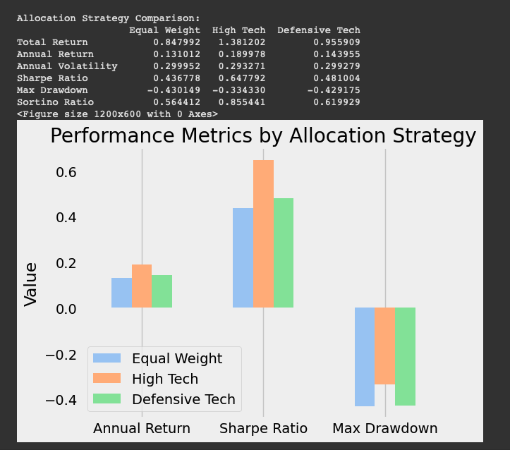

Conclusion

In this article, we’ve built a comprehensive portfolio backtesting framework that allows us to:

1. Simulate historical portfolio performance
2. Implement flexible rebalancing strategies
3. Calculate important performance metrics
4. Analyze drawdowns and recovery periods
5. Compare different allocation strategies
6. Visualize portfolio performance over time

Backtesting is a crucial step in portfolio management, as it helps us understand how our strategies would have performed historically. However, it’s important to remember that past performance doesn’t guarantee future results. Backtesting should be one of several tools in your investment decision-making process.

In future articles, we’ll explore more advanced topics such as factor investing, machine learning for portfolio optimization, and building a comprehensive portfolio management system.

Disclaimer: This analysis is for educational purposes only and not financial advice. Results are based on historical data from January 2023 to March 2025 and do not guarantee future performance. Investing involves risks, including the potential loss of principal. Consult a qualified financial advisor before making investment decisions.