6. Achieving Beta Neutrality in Your Investment Portfolio with Python

Beta neutrality is a powerful risk management strategy that can help protect your investments from broad market movements. In this article, I’ll walk you through how to analyze and neutralize the beta of a portfolio using Python, complete with code examples you can adapt for your own investments.

What is Beta Neutrality? 

Beta neutrality is a portfolio strategy that aims to eliminate market risk by constructing a portfolio with a net beta of zero. A beta of zero means the portfolio’s value is expected to be uncorrelated with the broader market’s movements. This strategy allows investors to focus on the specific performance of their stock selections, rather than being swayed by overall market trends.

Calculating Beta Neutrality with Python

Setting Up Our Environment

First, let’s import the necessary libraries:

import numpy as np
import pandas as pd
import yfinance as yf
import matplotlib.pyplot as plt
import seaborn as sns
from scipy import stats

Building Our Sample Portfolio

Let’s create a portfolio with five well-known stocks and download their historical data:

# Define our portfolio
tickers = ['AAPL', 'JPM', 'KO', 'TSLA', 'PG']
weights = np.array([0.2, 0.2, 0.2, 0.2, 0.2])  # Equal weights
portfolio_value = 50000  # $50,000 portfolio

# Download historical data
start_date = '2020-01-01'
end_date = '2024-12-31'
market_ticker = '^GSPC'  # S&P 500 index

# Get stock data
stock_data = yf.download(tickers + [market_ticker], start=start_date, end=end_date)['Close']

# Calculate daily returns
returns = stock_data.pct_change().dropna()

# Separate market returns
market_returns = returns[market_ticker]
stock_returns = returns[tickers]

Calculating Individual Stock Betas

Now, let’s calculate the beta for each stock in our portfolio:

# Calculate beta for each stock
betas = {}
for ticker in tickers:
    # Linear regression: stock returns vs market returns
    slope, intercept, r_value, p_value, std_err = stats.linregress(
        market_returns, stock_returns[ticker]
    )
    betas[ticker] = slope

# Create a DataFrame to display the betas
beta_df = pd.DataFrame(list(betas.items()), columns=['Stock', 'Beta'])
print("Individual Stock Betas:")
print(beta_df)

# Calculate portfolio beta
portfolio_beta = np.sum(weights * np.array(list(betas.values())))
print(f"\nPortfolio Beta: {portfolio_beta:.4f}")

This code calculates beta by running a linear regression of each stock’s returns against the market returns. The slope of this regression line is the beta. Below is the output return by the Python code:

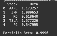
The portfolio has a beta of approximately 1, meaning that, overall, it carries roughly the same level of market risk as the market itself.

Visualizing Stock Correlations

Understanding correlations between stocks helps us assess diversification. Below part of the code plots a visualization of how the stocks correlate with each other:

# Calculate correlation matrix
correlation_matrix = stock_returns.corr()

# Plot the correlation matrix
plt.figure(figsize=(10, 8))
sns.heatmap(correlation_matrix, annot=True, cmap='coolwarm', vmin=-1, vmax=1)
plt.title('Stock Return Correlations')
plt.tight_layout()
plt.show()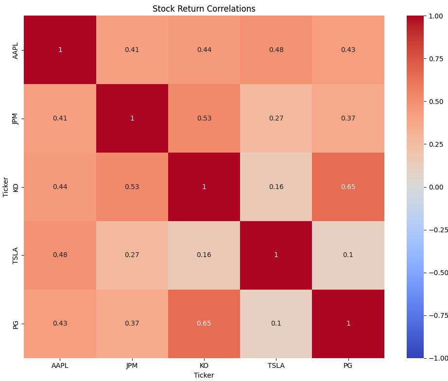

Calculating the Required Hedge

To make our portfolio beta-neutral, we need to determine the appropriate hedge. We can use below code in order to calculate how many SPY stocks we need to short in order to achieve portfolio neutrality:

# Calculate the market exposure we need to hedge
market_exposure_to_hedge = portfolio_value * portfolio_beta
print(f"Market exposure to hedge: ${market_exposure_to_hedge:.2f}")

# If using index futures or ETFs
spy_price = stock_data[market_ticker].iloc[-1]  # Latest S&P 500 price
print(f"Latest S&P 500 index value: ${spy_price:.2f}")

# If using SPY ETF (which tracks S&P 500)
spy_etf_price = 450  # Example price, in practice you'd fetch the current price
spy_shares_to_short = market_exposure_to_hedge / spy_etf_price
print(f"Number of SPY ETF shares to short: {spy_shares_to_short:.2f}")

The code returns below output:

• Market exposure to hedge: $49977.71. This value represents the portion of the portfolio’s value that is sensitive to market movements. In other words, given the portfolio’s current beta (which is 0.9996, very close to 1), it has $49977.71 exposed to the S&P 500’s fluctuations.

• Latest S&P 500 index value: $5906.94. This is the current price of the S&P 500 index at the time the code was run. It’s used as a reference point for calculating the hedge.

• Number of SPY ETF shares to short: 111.06. This is the key calculation. To hedge the market exposure of $49977.71, we would need to short 111.06 shares of the SPY ETF. By shorting these shares, we’re effectively taking a position that moves inversely to the market. This inverse movement offsets the market risk of your existing stock portfolio.

Using Options to Achieve Beta Neutrality

Now, let’s explore how to use put options to neutralize our portfolio’s beta instead of shorting ETF shares as we shown in the previous version:

def calculate_option_hedge(portfolio_value, portfolio_beta, spy_price,
                            option_delta, contract_multiplier=100):
    """
    Calculate the number of option contracts needed to hedge portfolio beta.

    Parameters:
    - portfolio_value: Total value of the portfolio
    - portfolio_beta: Beta of the portfolio
    - spy_price: Current price of SPY ETF
    - option_delta: Delta of the option (absolute value)
    - contract_multiplier: Number of shares per contract (typically 100)

    Returns:
    - Number of option contracts needed
    """
    # Market exposure to hedge
    market_exposure = portfolio_value * portfolio_beta

    # Value of one option contract at current price
    contract_value = spy_price * contract_multiplier

    # Number of contracts needed, adjusted for delta
    contracts_needed = market_exposure / (contract_value * option_delta)

    return contracts_needed

# Example: Using put options with a delta of -0.5
put_option_delta = 0.5  # Using absolute value for calculation
contracts_needed = calculate_option_hedge(
    portfolio_value, portfolio_beta, spy_etf_price, put_option_delta)
print(f"\nUsing put options with delta of -0.5:")
print(f"Number of put option contracts needed: {np.ceil(contracts_needed)}")

# Calculate the cost of the hedge
option_premium_per_share = 15  # Example premium
total_option_cost = np.ceil(contracts_needed) * option_premium_per_share * 100
print(f"Total cost of put options: ${total_option_cost:.2f}")
print(f"Hedge cost as percentage of portfolio: {(total_option_cost/portfolio_value)*100:.2f}%")

Below is the output and the interpretation of using put options with delta of -0.5 to hedge market risk:

Number of put option contracts needed: 3.0. This means that 3 put option contracts are required to hedge the portfolio’s market exposure. The output is actually 2.22, then it is up to us to decide if we want to round up to 3 or to 2 since we can’t buy fractions of contracts.

Total cost of put options: $4500. This is the total cost of buying the 3 put option contracts, based on an example premium per share.

Hedge cost as percentage of portfolio: 9.00%. This shows the cost of the hedge relative to the total portfolio value. In this case, it costs 9% of the portfolio value to implement the hedge.

Conclusion

Beta neutrality is a sophisticated strategy that can help protect your portfolio from market downturns while allowing you to capture returns from your stock selection. The Python code provided here gives you the tools to:

• Calculate individual stock and portfolio betas
• Visualize correlations between your holdings
• Determine the appropriate hedge size using index ETFs or options

Remember that maintaining beta neutrality requires regular monitoring and rebalancing as market conditions change. The options approach offers flexibility but comes with costs in terms of premiums and time decay.

Remember to have a look at my prior posts in order to find out how to use Python for portfolio management.

Disclaimer: Investing in financial markets involves risk, and past performance is not indicative of future results. The information provided in this article is for educational purposes only and should not be considered investment advice. It is essential to conduct thorough research and consult with a qualified financial advisor before making any investment decisions. The author and publisher disclaim any liability for any losses or damages that may arise from the use of this information.

Note: This article was drafted with the assistance of artificial intelligence and subsequently reviewed by the user to ensure accuracy and clarity.