4. Measuring Portfolio Sensitivity with Beta and Dollar Delta using Python

Understanding how your portfolio moves with the market—or against it—is key to managing risk and return effectively. In this post, we’ll dive into two powerful metrics using Python: Beta, which measures your portfolio’s sensitivity to market movements, and Dollar Delta, which quantifies the dollar impact of those movements. We’ll also calculate portfolio volatility and market correlation for a fuller picture. Building on our previous exploration of data analysis in Post 3: Data Analysis for Portfolio Management, where we fetched and analyzed stock data, we’ll use Python and real data from Apple (AAPL), Microsoft (MSFT), and Amazon (AMZN), benchmarked against the S&P 500 (SPY), to show you how to assess your portfolio’s behavior with hands-on examples.

Key Concepts

• Beta: Beta gauges how much your portfolio moves relative to the market. A Beta of 1 means it moves in lockstep with the market (e.g., S&P 500); above 1 means it’s more volatile; below 1, less volatile. For example, a Beta of 1.2 suggests a 20% bigger swing than the market.
• Dollar Delta: This translates Beta into dollars, showing how much your portfolio’s value changes for a $1 move in the market index. It’s a practical way to see real-world exposure.
• Portfolio Volatility: The standard deviation of returns, annualized, measures total risk—both market-driven and unique to your assets.
• Correlation to Market: This shows how closely your portfolio tracks the market, ranging from -1 (opposite movement) to 1 (perfect sync).

These metrics help you understand your portfolio’s risk profile and exposure to broader market trends.

Disclaimer: This article was drafted with the assistance of artificial intelligence and reviewed by the editor prior to publication to ensure accuracy and clarity.

Portfolio Beta with Python

We’ll use historical data from January 1, 2023, to March 14, 2025 (today’s date), for a portfolio of AAPL, MSFT, and AMZN with equal weights (1/3 each), compared to SPY as the market proxy. Here’s the plan:

1. Fetch Data: Download adjusted closing prices for the stocks and SPY.
2. Calculate Returns: Compute daily returns for the portfolio and market.
3. Compute Beta: Use regression or covariance to find the portfolio’s Beta relative to SPY.
4. Estimate Dollar Delta: Multiply Beta by the portfolio’s value to see dollar exposure.
5. Add Volatility and Correlation: Calculate annualized volatility and market correlation.

import yfinance as yf
import pandas as pd
import numpy as np
import matplotlib.pyplot as plt

# Define stocks, market proxy, and period
tickers = ['AAPL', 'MSFT', 'AMZN']
market_ticker = 'SPY'
start_date = '2023-01-01'
end_date = pd.Timestamp.today().strftime('%Y-%m-%d') # Use today's date

# Fetch adjusted closing prices
data = yf.download(tickers + [market_ticker], start=start_date, end=end_date)['Close']
# Calculate daily percentage returns and drop NaN values
returns = data.pct_change().dropna()

# Portfolio returns (equal weights: 1/3 each)
weights = np.array([1/len(tickers)] * len(tickers))
portfolio_returns = returns[tickers].dot(weights)

# Market returns
market_returns = returns[market_ticker]

# Step 1: Calculate Beta
# Calculate covariance between portfolio returns and market returns
covariance = np.cov(portfolio_returns, market_returns)[0, 1]
# Calculate variance of market returns
market_variance = np.var(market_returns)
# Calculate Beta by dividing covariance by market variance
beta = covariance / market_variance
print(f"Portfolio Beta: {beta:.4f}")

# Step 2: Dollar Delta (assume $10,000 portfolio)
portfolio_value = 10000
# Calculate Dollar Delta by multiplying Beta by portfolio value
dollar_delta = beta * portfolio_value
print(f"Dollar Delta (per $1 move in SPY): ${dollar_delta:.2f}")

# Step 3: Portfolio Volatility (annualized)
# Calculate standard deviation of portfolio returns and annualize it
portfolio_vol = portfolio_returns.std() * np.sqrt(252)
print(f"Annualized Portfolio Volatility: {portfolio_vol:.4f}")

# Step 4: Correlation to Market
# Calculate correlation coefficient between portfolio returns and market returns
correlation = np.corrcoef(portfolio_returns, market_returns)[0, 1]
print(f"Correlation to SPY: {correlation:.4f}")

# Visualization: Portfolio vs. Market Returns (Cumulative Value)
plt.figure(figsize=(10, 6))
plt.plot((1 + portfolio_returns).cumprod() * portfolio_value, label='Portfolio ($10,000)')
plt.plot((1 + market_returns).cumprod() * portfolio_value, label='SPY ($10,000)')
plt.title('Portfolio vs. Market Performance (Cumulative Value)')
plt.xlabel('Date')
plt.ylabel('Value ($)')
plt.legend()
plt.show()

# Visualization: Portfolio vs. Market Returns (Percentage Returns)
plt.figure(figsize=(10, 6))
plt.plot(portfolio_returns.cumsum(), label='Portfolio Cumulative Returns')
plt.plot(market_returns.cumsum(), label='SPY Cumulative Returns')
plt.title('Portfolio vs. Market Performance (Cumulative Percentage Returns)')
plt.xlabel('Date')
plt.ylabel('Cumulative Percentage Returns')
plt.legend()
plt.show()

The code above should give you something similar to below:

Interpretation of the results of our portfolio versus SPY

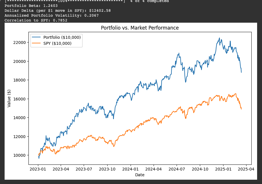
1. Portfolio Beta (1.2403)
   • A Beta of 1.2403 indicates that your portfolio is approximately 24% more volatile than the S&P 500 (SPY). This means that if SPY rises or falls by 1%, your portfolio is expected to move by about 1.24% in the same direction, assuming other factors remain constant.
2. Dollar Delta ($124 per 1% move in SPY)
   • For a $10,000 portfolio with a beta of 1.24, a 1% move in SPY should translate to roughly a $124 move in the portfolio.
3. Annualized Portfolio Volatility (0.2067 or 20.67%)
   • The annualized volatility of 20.67% indicates the portfolio’s overall risk level, capturing both market-driven and stock-specific fluctuations. Compared to SPY’s typical volatility (around 15-18%), this is moderately higher, aligning with the tech sector’s inherent volatility.
4. Correlation to SPY (0.7852)
   • A correlation of 0.7852 shows that your portfolio moves in strong alignment with the market, but not perfectly. This indicates that about 78.5% of your portfolio’s movement is explained by SPY, with the remainder due to stock-specific factors (e.g., company earnings or sector trends). The imperfect correlation offers some diversification benefits but still ties the portfolio closely to market performance.
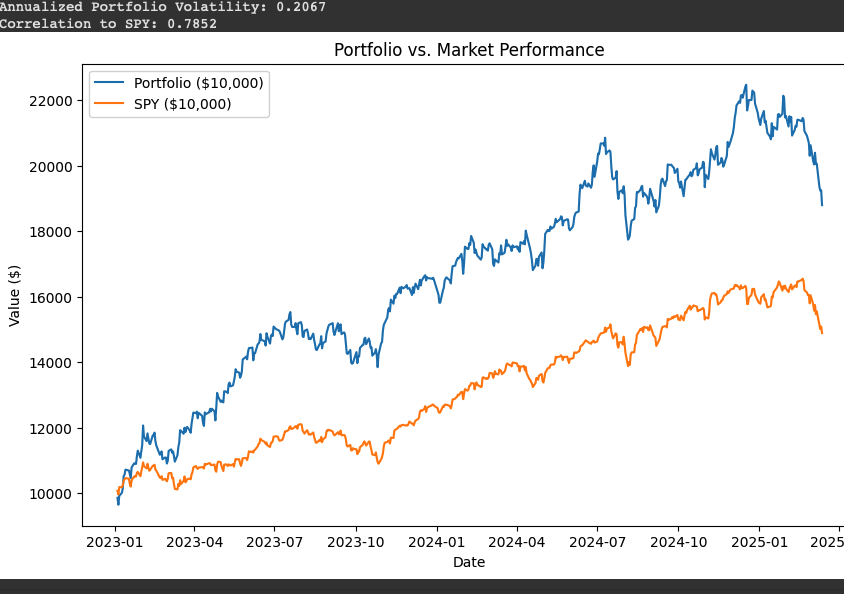
5. Portfolio vs. Market Performance Graph
   • The graph shows the growth of a $10,000 investment in your portfolio (blue line) versus SPY (orange line) from January 2023 to March 2025. Both lines trend upward initially, reflecting a bullish market, but the portfolio outpaces SPY early on, likely due to tech stock gains. However, a noticeable dip toward the end (around late 2024 to early 2025) suggests a period of underperformance or increased volatility, possibly due to market corrections or tech sector challenges. The portfolio’s higher Beta (1.24) amplifies these swings compared to SPY.

Conclusion with Actionable Takeaways

These metrics provide a clear picture of your portfolio’s behavior:

• Leverage Beta: A Beta of 1.24 indicates a growth tilt. If you’re comfortable with this risk, it’s a good fit for bullish markets. To reduce exposure, consider adding lower-Beta assets like utilities (e.g., Duke Energy, DUK) or bonds.
• Assess Volatility: At 20.67%, your volatility is manageable but higher than the market. If this exceeds your risk tolerance, diversify with less volatile assets or hedge with options.
• Optimize Correlation: The 0.7852 correlation suggests room to add uncorrelated assets (e.g., gold or real estate ETFs) to reduce market dependency.
• Review Performance Trends: The graph’s dip toward 2025 warrants attention. Re-run the analysis with updated data to see if this is a short-term correction or a trend, adjusting your strategy accordingly.

Disclaimer: This analysis is for educational purposes only and not financial advice. Results are based on historical data from January 2023 to March 2025 and do not guarantee future performance. Investing involves risks, including the potential loss of principal. Consult a qualified financial advisor before making investment decisions.